Quadratic Circuit Hamiltonians: Counter-Rotating Terms, RWA, and Downfolding
Node role: Concept.
Reader task: Start from one linear circuit’s stored energy, understand why both \(\mathbf h\) and \(\boldsymbol\Delta\) appear, and decide whether an RWA or downfolded model is accurate enough for a named observable.
This page explains a downstream quantum/quantization representation. Its \(\mathbf h\), \(\boldsymbol\Delta\), RWA, and Bogoliubov objects do not define classical anchored-bare open-EOM roots, a response fit, or a design objective. It is generic theory, not a claim that a particular package implements it.
Prerequisites and source scope
Start with independent physical flux coordinates and the conservative circuit Hamiltonian. The flux-to-mode symbol bridge distinguishes classical amplitudes from operators and their expectations.
Reorganized source explanation: node-flux quantization follows (Vool and Devoret 2017); canonical normal forms and Bogoliubov transformations follow (Kustura et al. 2019); controlled bosonic downfolding has the additional canonical structure discussed in (Massarelli et al. 2022). This-page derivation: the local normalization, exchange/pairing coefficient map, two-mode second-order shifts, and displayed Schur identities are derived below in the stated convention. The citations do not establish equality with a fitted open-response coupling or prescribe a design tolerance.
Build a picture before the matrices
What changes when a second coordinate is coupled to the first? One parabolic potential has one curvature. Two uncoupled coordinates have circular equal-energy contours when their scales match. Coupling can tilt and stretch those contours: the collective stiff and soft directions need not follow either original coordinate axis.
We will reuse one public analytical example throughout the pictures. Define dimensionless canonical quadratures
\[ x_j=\frac{a_j+a_j^\dagger}{\sqrt2},\qquad p_j=\frac{a_j-a_j^\dagger}{i\sqrt2},\qquad [x_j,p_k]=i\delta_{jk}, \]
and the two-coordinate Hamiltonian
\[ \frac{H}{\hbar\omega_0} =\frac{p_a^2+p_b^2+x_a^2+x_b^2}{2}+2\eta x_a x_b. \]
Here both bare frequencies are \(\omega_0\) and the exchange and pairing coefficients are \(g=d=\eta\omega_0\). The quadrature expression includes the constant zero-point offset; it may be dropped consistently in ladder-operator notation without changing frequency differences. This is the position-coupled specialization of the quadratic model discussed by (Heib et al. 2025, sec. I.2, Eq. (1)); the following contour and frequency identities are this-page analytical derivations, not package output or measurements.
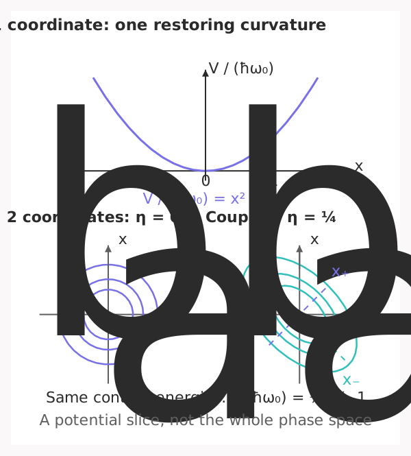
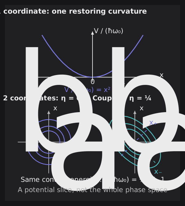
How to read it: at \(\eta=1/4\), the directions \(x_\pm=(x_a\pm x_b)/\sqrt2\) have curvatures \(1\pm2\eta\). The shorter contour axis is the stiffer \(x_+\) direction. This rotation is only part of a canonical normal-mode construction: the momenta transform too, and the new oscillator scales require normalization. A potential contour alone does not display the full phase-space Hamiltonian or its quantum correlations. Open the vector figure at full sizeOpen the vector figure at full size.
The positive-definite domain is \(|\eta|<1/2\), a mathematical property of this model, not a research admission criterion. The pictures use \(\eta=0\) and \(1/4\); the later plot shows a pedagogical interval inside that domain. No search range or approximation-accuracy threshold is being prescribed.
The conclusion first
The physical starting point is one quadratic electromagnetic energy:
\[ \boxed{ H =\frac12\vec Q^{\mathsf T}\mathbf C^{-1}\vec Q +\frac12\vec\Phi^{\mathsf T}\mathbf K_\Phi\vec\Phi. } \]
For the real reciprocal matrices used throughout this node, writing that same energy with local oscillator operators produces two real symmetric matrices at the same time:
\[ \boxed{ \frac H\hbar =\vec a^\dagger\mathbf h\vec a +\frac12\left( \vec a^T\boldsymbol\Delta\vec a +\vec a^{\dagger T}\boldsymbol\Delta\vec a^\dagger \right)+\text{constant}. } \]
- \(\mathbf h\) is the number-conserving block. It exists before any RWA.
- \(\boldsymbol\Delta\) is the pairing, counter-rotating, or antiresonant block.
- The number-conserving/pairing RWA used here keeps \(\mathbf h\) and neglects \(\boldsymbol\Delta\).
- Exact normal-mode diagonalization keeps both blocks and changes basis.
- Downfolding removes declared high-frequency coordinates while retaining their frequency-dependent virtual loading.
These are different operations. None creates or deletes a physical capacitor or inductor.
Throughout this page, \(\boldsymbol\Delta\) is a bold matrix pairing block. A scalar \(\Delta\) elsewhere in the Knowledge Base denotes a detuning; the two symbols must not be interchanged.
1 — Start from electric and magnetic stored energy
In a declared generalized-flux basis, let
\[ \mathbf A_Q:=\mathbf C^{-1}, \qquad \mathbf B_\Phi:=\mathbf K_\Phi. \]
The charge term is the electric energy and the flux term is the magnetic energy. This is the circuit Hamiltonian before choosing oscillator operators. The construction follows the node-flux circuit quantization reviewed by (Vool and Devoret 2017). Assume a finite, static, reciprocal conservative model on independent coordinates, with real symmetric positive-definite \(\mathbf C\) and \(\mathbf K_\Phi\) on the oscillator subspace. Losses and frequency-dependent response fits are not silently treated as stored-energy coefficients.
Choose one positive local impedance scale for each retained coordinate,
\[ Z_i=\sqrt{\frac{(A_Q)_{ii}}{(B_\Phi)_{ii}}}, \qquad \mathbf Z=\operatorname{diag}(Z_i), \]
This local normalization requires \((A_Q)_{ii}>0\) and \((B_\Phi)_{ii}>0\). A free coordinate with no restoring term is not a local harmonic oscillator; it must remain explicit or be reduced under a declared boundary before this normalization is used.
The canonical operators are then
\[ \hat\Phi_i=\sqrt{\frac{\hbar Z_i}{2}} (\hat a_i+\hat a_i^\dagger), \qquad \hat Q_i=-i\sqrt{\frac{\hbar}{2Z_i}} (\hat a_i-\hat a_i^\dagger). \]
This is a change of coordinates, not an approximation. The operators \(a_i\) still label the declared local bare directions; they are not yet the exact normal modes.
Anchored impedance scaling and normal-mode normalization are different
Basis direction and normalization are separate choices:
| Operation | Does it mix subsystem directions? | Result |
|---|---|---|
| Anchored impedance normalization | No | Scales each retained \((\Phi_i,Q_i)\) pair into the local oscillator \(a_i\) and preserves its named coordinate identity |
| Conservative normal-mode transform | Yes | Rotates the complete closed circuit into collective eigenvectors |
The chosen local impedance is not arbitrary bookkeeping. It equalizes the diagonal charge- and flux-energy coefficients,
\[ \left[\mathbf Z^{-1/2}\mathbf A_Q\mathbf Z^{-1/2}\right]_{ii} = \left[\mathbf Z^{1/2}\mathbf B_\Phi\mathbf Z^{1/2}\right]_{ii} =\omega_i, \]
and therefore makes \([\boldsymbol\Delta]_{ii}=0\). It is a diagonal canonical scaling, not a diagonalization; off-diagonal \(h_{ij}\) and \(\Delta_{ij}\) generally remain.
For closed normal modes, a dimensionless eigenvector matrix \(\mathbf U\) may instead retain physical flux coordinates through
\[ \boxed{ \mathbf K_\Phi\mathbf U =\mathbf C\mathbf U\boldsymbol\Omega_{\rm N}^2, \qquad \vec\Phi=\mathbf U\vec\Phi_{\rm N}. } \]
Choosing the column scale of \(\mathbf U\) then gives
\[ \mathbf U^T\mathbf C\mathbf U =\mathbf C_{\rm N}=\operatorname{diag}(C_\mu), \qquad \mathbf U^T\mathbf K_\Phi\mathbf U =\mathbf C_{\rm N}\boldsymbol\Omega_{\rm N}^2. \]
Then \(\Phi_{\mu,\rm N}\) remains in webers and \(Z_\mu=1/(\omega_\mu C_\mu)\). The commonly used mathematical \(\mathbf C\)-normalized eigenvectors set the metric to \(\mathbf I\) by absorbing \(\mathbf C_{\rm N}^{1/2}\) into the coordinates; those mass-weighted coordinates are not themselves weber-valued node or generalized fluxes.
2 — Why \(\mathbf h\) and \(\boldsymbol\Delta\) appear together
Previous: classical amplitudes and operator promotion · Next: RWA, Bogoliubov, and normal modes
Define the charge- and flux-energy contributions in oscillator units:
\[ \boxed{ \mathbf X :=\mathbf Z^{-1/2}\mathbf A_Q\mathbf Z^{-1/2}, \qquad \mathbf Y :=\mathbf Z^{1/2}\mathbf B_\Phi\mathbf Z^{1/2}. } \]
The matrices \(\mathbf X\), \(\mathbf Y\), \(\mathbf h\), and \(\boldsymbol\Delta\) have angular-frequency units (\(\mathrm{s}^{-1}\)); \(H/\hbar\) is not a cyclic-frequency Hamiltonian. Throughout, \(\mathsf T\) (or \(T\)) means ordinary transpose, \(*\) means complex conjugation, and \(\dagger\) means adjoint. Here the coefficient matrices are real symmetric, so \(\mathbf h^\dagger=\mathbf h\) and \(\boldsymbol\Delta^{\mathsf T}=\boldsymbol\Delta\); this does not make transpose and adjoint interchangeable for general complex coefficients.
Direct substitution gives
\[ \boxed{ \mathbf h=\frac{\mathbf X+\mathbf Y}{2}, \qquad \boldsymbol\Delta=\frac{\mathbf Y-\mathbf X}{2}. } \]
For \(i\ne j\), this stated \(\mathbf A_Q/\mathbf B_\Phi\) convention calls the two exact fixed-anchored-basis coefficients
\[ \boxed{ J_{\rm ex,ij}=h_{ij} =\frac12\left[ \frac{(A_Q)_{ij}}{\sqrt{Z_iZ_j}} +(B_\Phi)_{ij}\sqrt{Z_iZ_j} \right], \qquad \Lambda_{ij}=\Delta_{ij} =\frac12\left[ -\frac{(A_Q)_{ij}}{\sqrt{Z_iZ_j}} +(B_\Phi)_{ij}\sqrt{Z_iZ_j} \right]. } \]
For each unordered pair \(i<j\), \(H/\hbar\) contains
\[ J_{\rm ex,ij}(a_i^\dagger a_j+a_j^\dagger a_i) +\Lambda_{ij}(a_i a_j+a_i^\dagger a_j^\dagger). \]
Both coefficients are exact full-quadratic coefficients only in this fixed anchored basis and stated sign/phase convention. Do not transplant these signs or factors to another convention without rederiving the map.
\(J_{\rm H}\) is an alternative name for this same full-Hamiltonian exchange coefficient: \(J_{\rm H}=J_{\rm ex}\) here. It is not a fourth coupling. After an explicitly stated RWA drops \(\Lambda\), the inherited reduced coefficient is \(J_{\rm RWA}=J_{\rm ex}\) numerically, but that equality does not make the \(N\)-dimensional reduced model exact.
An observed avoided-crossing half-splitting is instead
\[ J_{\rm split}=\frac{\omega_+-\omega_-}{2}. \]
It is an observable derived from two hybridized frequencies, not a definition of \(J_{\rm ex}\), \(J_{\rm H}\), \(J_{\rm RWA}\), or an open-system local-response coupling. Equality needs separately stated assumptions such as a resonant, lossless, two-mode, number-conserving model with the relevant coordinates and no competing shifts.
The inverse bridge back to the circuit matrices is therefore
\[ \boxed{ \mathbf h-\boldsymbol\Delta =\mathbf Z^{-1/2}\mathbf A_Q\mathbf Z^{-1/2}, \qquad \mathbf h+\boldsymbol\Delta =\mathbf Z^{1/2}\mathbf K_\Phi\mathbf Z^{1/2}. } \]
Thus \(\mathbf h\) and \(\boldsymbol\Delta\) together retain the complete quadratic stored energy in this normalization. Keeping only \(\mathbf h\) is the RWA; it is not an invertible reconstruction of the original \(\mathbf C,\mathbf K_\Phi\) model.
Frequencies, probe detuning, and the exact first-order operator
The matrix \(\mathbf h\) has angular-frequency units. Its diagonal entries \(h_{ii}\) are local oscillator frequency coefficients, while its off-diagonal entries \(h_{ij}\) are exchange angular rates. These local coefficients are not in general the exact coupled normal-mode frequencies. In the number-conserving reduction, a frequency-domain driven equation contains
\[ (\mathbf h-\omega\mathbf I)\vec a(\omega)=\text{drive}. \]
Its diagonal entries \(h_{ii}-\omega\) are probe–mode detunings. They are not the mode–mode detuning \(h_{ii}-h_{jj}\) between two internal modes.
For a general quadratic system with pairing, the exact linear first-order problem is instead the \(2N\)-dimensional Nambu/phase-space operator,
\[ \left[ \begin{pmatrix} \mathbf h & \boldsymbol\Delta\\ -\boldsymbol\Delta^* & -\mathbf h^* \end{pmatrix} -\omega\mathbf I_{2N} \right] \begin{pmatrix}\vec a\\\vec a^\dagger\end{pmatrix} =\text{drive}. \]
The \(N\)-dimensional \(\mathbf h-\omega\mathbf I\) form is exact only when \(\boldsymbol\Delta=0\), or after an explicitly stated number-conserving/RWA reduction. It must not be presented as the exact paired system.
For the response-side local coupling and its distinct assumptions, see Which coupling is this?.
This is the missing bridge from electromagnetic stored energy to the two oscillator blocks:
| Physical contribution | Contribution to \(h_{ij}\) | Contribution to \(\Delta_{ij}\) |
|---|---|---|
| Charge/electric coupling \(X_{ij}\) | \(+X_{ij}/2\) | \(-X_{ij}/2\) |
| Flux/magnetic coupling \(Y_{ij}\) | \(+Y_{ij}/2\) | \(+Y_{ij}/2\) |
Therefore, for one off-diagonal pair \(i\ne j\),
\[ Y_{ij}=0 \quad\Longrightarrow\quad \Delta_{ij}=-h_{ij} \qquad\text{(pure capacitive coupling)}, \]
whereas
\[ X_{ij}=0 \quad\Longrightarrow\quad \Delta_{ij}=+h_{ij} \qquad\text{(pure inductive coupling)}. \]
If both electric and magnetic paths exist, neither sign relation is general. The two contributions can reinforce or partly cancel in either block.
\(\mathbf h\) and \(\boldsymbol\Delta\) describe the chosen local oscillator basis. A stable closed linear circuit can instead be transformed to its exact normal modes; in that basis the quadratic Hamiltonian is diagonal and has no pairing block. The invariant physical results are the complete response and normal-mode frequencies, not one isolated entry such as \(\Delta_{ij}\).
Before choosing an approximation, first identify the question:
| Question | Operation |
|---|---|
| What are the exact closed frequencies? | Diagonalize the complete conservative quadratic Hamiltonian. |
| What is the narrow-band number-conserving model? | Apply a declared RWA and validate its response window. |
| What is the low-frequency effect of retained high coordinates? | Downfold them through a frequency-dependent self-energy. |
RWA, exact Bogoliubov diagonalization, and downfolding solve different problems; none is a synonym for either of the others.
3 — What the two blocks do
For two coordinates \(i\) and \(j\), the off-diagonal terms are
\[ h_{ij}(a_i^\dagger a_j+a_i a_j^\dagger) +\Delta_{ij}(a_i^\dagger a_j^\dagger+a_i a_j). \]
The \(h_{ij}\) term exchanges one excitation between the two local coordinates. The \(\Delta_{ij}\) term connects states whose total local excitation number differs by two. It is often called a pairing or two-mode-squeezing term.
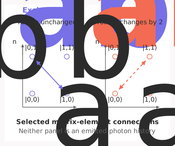
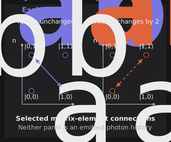
How to read it: \(a_a^\dagger a_b\) moves one occupation from \(b\) to \(a\); \(a_a^\dagger a_b^\dagger\) raises both. The displayed connections have matrix elements \(h_{ab}\) and \(\Delta_{ab}\) respectively. They are selected entries of the full occupation-space Hamiltonian, not a Hilbert-space truncation or a sequence of emissions. Equal coefficients in our \(g=d\) example do not mean equal operator actions. Open the vector figureOpen the vector figure.
For a stable, static, passive circuit, \(\boldsymbol\Delta\ne0\) does not mean that the circuit continuously creates measurable photons. It means the vacuum defined by the local \(a_i\) operators is not the exact ground state. The exact normal-mode vacuum is related to it by a Bogoliubov transformation.
4 — What the rotating-wave approximation removes
Previous: \(\mathbf h\) and \(\boldsymbol\Delta\) · Related: open-response versus Hamiltonian coupling
Use the uncoupled evolution
\[ H_0=\sum_i\hbar\omega_i a_i^\dagger a_i. \]
In its interaction picture,
\[ a_i^\dagger a_j \propto e^{+i(\omega_i-\omega_j)t}, \qquad a_i a_j \propto e^{-i(\omega_i+\omega_j)t}. \]
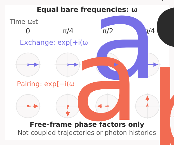
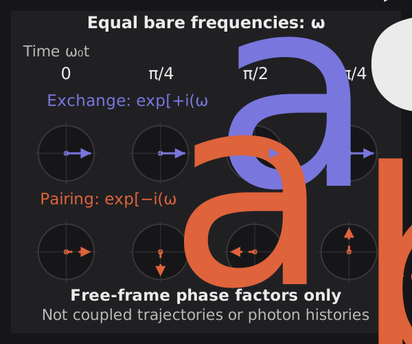
How to read it: in the resonant example \(\omega_a=\omega_b=\omega_0\), the difference phase is exactly one, while the sum phase is \(e^{-2i\omega_0t}\). Contributions with changing phase can average away on a longer time scale; the constant exchange factor cannot be discarded by that same argument. This picture motivates the approximation, not a universal error bound. Open the vector figureOpen the vector figure.
Near an \(i\)–\(j\) resonance, the exchange term varies with the small frequency difference, while the pairing term varies with the large frequency sum. The RWA averages out the latter and uses
\[ \boxed{ H_{\rm RWA}=\hbar\vec a^\dagger\mathbf h\vec a. } \]
This number-conserving/pairing RWA is therefore a time-scale approximation in a declared basis. It is not the statement that the magnetic or electric part of the stored energy has disappeared. A later secular or dispersive approximation may additionally neglect far-detuned entries of \(\mathbf h\); that is a separate step. Quantitative bounds for coupled oscillators require both a coupling ratio and an observation time or error tolerance; see (Heib et al. 2025).
Useful screening scales are
\[ \epsilon_{ij}^{(\rm pair)} =\left|\frac{\Delta_{ij}}{\omega_i+\omega_j}\right|, \qquad \delta\omega_{ij}^{(\rm pair)} \sim\left|\frac{\Delta_{ij}^2}{\omega_i+\omega_j}\right|. \]
The first estimates perturbative smallness. The second estimates the frequency shift scale; neither expression is an automatic accuracy threshold. To assess an approximation for a named observable, compare the complete and RWA models in the relevant frequency/time regime. Any application-specific tolerance belongs to that application, not to this generic derivation.
5 — Exact conservative result: Bogoliubov diagonalization
For the real passive matrices used here, the exact doubled Heisenberg EOM is
\[ \boxed{ i\frac{d}{dt} \begin{pmatrix}\vec a\\\vec a^\dagger\end{pmatrix} = \underbrace{ \begin{pmatrix} \mathbf h&\boldsymbol\Delta\\ -\boldsymbol\Delta&-\mathbf h^T \end{pmatrix}}_{\mathcal L_{\rm BdG}} \begin{pmatrix}\vec a\\\vec a^\dagger\end{pmatrix}. } \]
A canonical Bogoliubov transformation mixes \(a\) and \(a^\dagger\) while preserving their commutators. When the circuit is dynamically stable, the positive eigenfrequencies of \(\mathcal L_{\rm BdG}\) are its exact conservative normal-mode frequencies. This is the appropriate exact treatment described by (Kustura et al. 2019).
The local diagonal \(h_{ii}\) is consequently a coefficient in one declared basis. It is not, by itself, a basis-independent resonance frequency. Exact normal-mode frequencies may instead be obtained directly from the classical linear response, as used in black-box circuit quantization (Nigg et al. 2012).
What does dropping pairing change?
Return to the same resonant example, with \(g=d=\eta\omega_0\). Rotating both \(x\) and \(p\) to symmetric/antisymmetric coordinates separates the two quadratic directions; the corresponding oscillator normalization then gives the exact full frequencies
\[ \frac{\Omega_\pm}{\omega_0}=\sqrt{1\pm2\eta}. \]
Dropping pairing but keeping the same exchange coefficient gives instead
\[ \frac{\Omega_{\pm,\mathrm{RWA}}}{\omega_0}=1\pm\eta. \]
The labels \(+\) and \(-\) identify the symmetric and antisymmetric directions, not arbitrary sorted eigenstate indices. These closed-form results use the declared model, not an eigensolver or a fitted response.
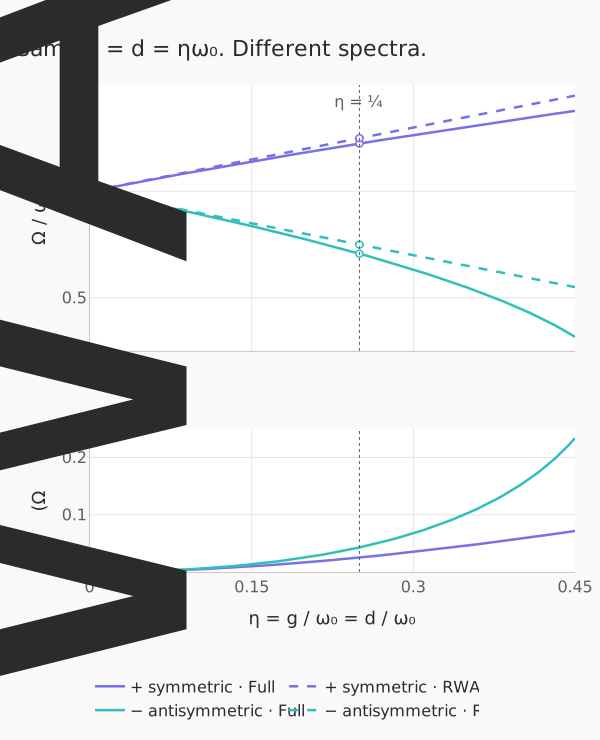
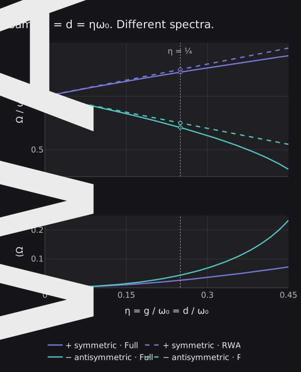
How to read it: all four curves meet at zero coupling, but removing pairing changes both frequencies. At the marked \(\eta=1/4\):
| Fixed branch | Exact full \(\Omega/\omega_0\) | RWA \(\Omega/\omega_0\) |
|---|---|---|
| Symmetric \(+\) | \(\sqrt{3/2}\approx1.2247\) | \(1.25\) |
| Antisymmetric \(-\) | \(\sqrt{1/2}\approx0.7071\) | \(0.75\) |
The residuals are approximately \(0.0253\omega_0\) and \(0.0429\omega_0\), respectively. They are consequences of this analytical example, not an accuracy tolerance or a performance claim. Open the vector plotOpen the vector plot.
This resonant comparison does not use the nondegenerate perturbation formula in the next section: its exchange denominator would vanish here. Keep that nonresonant approximation separate from this exact example.
6 — Two-mode frequency renormalization
Consider one low mode \(p\) and one high mode \(c\):
\[ \frac H\hbar =\omega_p a_p^\dagger a_p +\omega_c a_c^\dagger a_c +g(a_p^\dagger a_c+a_pa_c^\dagger) +d(a_p^\dagger a_c^\dagger+a_pa_c). \]
To second order,
\[ \boxed{ \delta\omega_p \simeq \frac{g^2}{\omega_p-\omega_c} -\frac{d^2}{\omega_p+\omega_c}. } \]
The first term comes from the virtual exchange path \(|1_p,0_c\rangle\rightarrow|0_p,1_c\rangle\). The pairing term shifts both the ground and excited states:
\[ \frac{\delta E_0}{\hbar}=-\frac{d^2}{\omega_p+\omega_c}, \qquad \frac{\delta E_1}{\hbar}=-\frac{2d^2}{\omega_p+\omega_c}. \]
Subtracting the ground-state shift from the excited-state shift gives the second term in \(\delta\omega_p\). This is a counter-rotating or antiresonant frequency renormalization. It is related to Bloch–Siegert physics, but that more specific name should not be used as a universal synonym.
The estimate requires
\[ |g|\ll|\omega_c-\omega_p|, \qquad |d|\ll\omega_c+\omega_p, \]
and a stable quadratic Hamiltonian. Otherwise solve the full BdG problem.
7 — Downfolding a high mode is not the RWA
Partition the exact doubled vector into retained low coordinates \(L\) and eliminated high coordinates \(H\), keeping every annihilation operator together with its creation partner:
\[ \boldsymbol\Psi_L :=\begin{pmatrix}\vec a_L\\\vec a_L^\dagger\end{pmatrix}, \qquad \boldsymbol\Psi_H :=\begin{pmatrix}\vec a_H\\\vec a_H^\dagger\end{pmatrix}. \]
Let \(\mathcal D(\omega)\) be the complete doubled dynamic matrix. For a closed, frequency-independent Hamiltonian,
\[ \mathcal D(\omega)=\omega\mathbf I-\mathcal L_{\rm BdG}. \]
For an open circuit, \(\mathcal D(\omega)\) must also contain the declared bath self-energy and port boundary. In either case, write
\[ \begin{pmatrix} \mathcal D_{LL}&\mathcal D_{LH}\\ \mathcal D_{HL}&\mathcal D_{HH} \end{pmatrix} \begin{pmatrix}\boldsymbol\Psi_L\\\boldsymbol\Psi_H\end{pmatrix}=0. \]
Where \(\mathcal D_{HH}(\omega)\) is invertible, eliminating \(\boldsymbol\Psi_H\) gives
\[ \boxed{ \mathcal D_{L,\rm eff}(\omega) =\mathcal D_{LL} -\mathcal D_{LH}\mathcal D_{HH}^{-1}\mathcal D_{HL}. } \]
Define the downfolding self-energy by
\[ \boxed{ \boldsymbol\Sigma_{L,\rm down}(\omega) :=\mathcal D_{LH}\mathcal D_{HH}^{-1}\mathcal D_{HL}, \qquad \mathcal D_{L,\rm eff} =\mathcal D_{LL}-\boldsymbol\Sigma_{L,\rm down}. } \]
This exact self-energy is generally frequency-dependent. It can change:
- low-coordinate diagonal frequencies;
- low–low coherent couplings;
- the low-coordinate pairing block;
- port participation and, when the eliminated block is open, linewidths.
It contains both difference-frequency exchange denominators and sum-frequency counter-rotating denominators. A controlled low-energy Schrieffer–Wolff reduction of a bosonic BdG system must preserve its symplectic structure; see (Massarelli et al. 2022).
A constant matrix such as
\[ \mathbf h_{\rm eff}^{(L)} \]
is allowed only after declaring the expansion frequency, bandwidth, retained order, residual pairing, and response error. It is a narrow-band effective model, not an exact identity. Drive, observation, and bath maps must follow the same elimination when an observable is compared; a reduced dynamic matrix alone is not the complete port response.
8 — Keep three operations separate
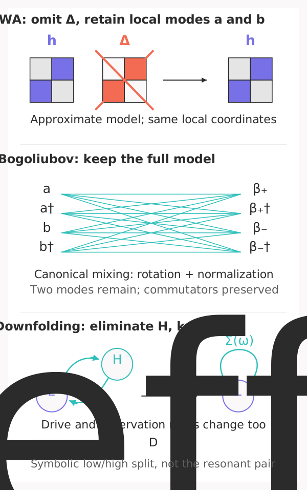
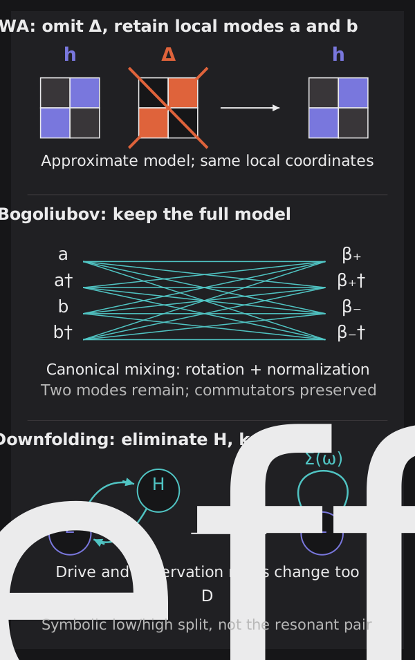
How to read it: crossing out a block, changing representation, and eliminating variables are not the same arrow. The normal-mode map includes creation/annihilation mixing and normalization, not only the contour rotation. The low/high partition in the last panel is symbolic: the resonant pair used in the frequency plot does not supply a separated high mode to eliminate. Open the vector comparisonOpen the vector comparison.
| Operation | What is removed? | What remains? | Output |
|---|---|---|---|
| RWA | Pairing terms in one chosen oscillator description | All coordinates and \(\mathbf h\) | Approximate number-conserving Hamiltonian |
| Dynamic downfolding | Declared high dynamic coordinates | Their virtual loading and mediated coupling | Frequency-dependent self-energy |
| Static circuit-matrix reduction | Declared algebraic/internal coordinates under a quasistatic zero-injection boundary | Their static loading | Schur-complemented circuit matrix |
The two reduction rows use the same Schur-complement algebra on different operators and boundaries. Network theory may also call a frequency-domain Schur reduction a dynamic Kron reduction. The word static here names only the \(\mathbf C\), \(\mathbf K_\Phi\), or zero-frequency specialization; it does not redefine all Kron reduction as static. Applying either reduction does not imply an RWA.
Interpreting a reduced model
Keep the retained/eliminated partition, normalization, expansion point and frequency window explicit when reporting a reduced model. A full conservative quadratic calculation and an open-system response answer different questions: losses, ports, and the bath self-energy must be supplied to predict open poles, linewidths, or \(S/Y/Z\). Do not promote \(h_{ij}\), a pole half-splitting, or a fitted open-response coupling into interchangeable observables.
There is no universal RWA accuracy or downfolding tolerance on this page. Comparison with the complete model can diagnose approximation error for the chosen observable; acceptance criteria remain application-owned.
Connections
- Physical circuit coordinates and open-EOM reduction establishes the independent coordinates, open operator, and boundary.
- Circuit Lagrangian, Hamiltonian, and canonical quantization establishes the conservative stored-energy and canonical starting point.
- Normalization and coupling meanings distinguishes fixed-basis coefficients from local open-response couplings.
- Poles, zeros, and residues defines local response normalization, not a universal Hamiltonian map.
- Schur complement and Kron reduction explains the elimination algebra and its boundary.
References
- (Vool and Devoret 2017): circuit energy, independent coordinates, and canonical quantization.
- (Kustura et al. 2019): quadratic canonical normal forms and stable Bogoliubov diagonalization.
- (Heib et al. 2025): bounds on RWA dynamics for coupled harmonic oscillators; not a universal design threshold.
- (Massarelli et al. 2022): structure-preserving Schrieffer–Wolff treatment of bosonic BdG systems.
- (Nigg et al. 2012): the role of classical linear modes in black-box circuit quantization, not a proof that a response fit supplies every quantum coefficient.
| Field | Value |
|---|---|
| Status | Source-backed |
| Semantic role | Derive exchange and pairing blocks from one conservative quadratic energy and distinguish RWA, canonical diagonalization, and downfolding. |
| Used by | Normalization, Symbol conventions, and Physical coordinates. |
| Open review question | Can a reader reconstruct both energy blocks and explain which approximation drops pairing, changes basis, or eliminates coordinates without confusing a coefficient with a response observable? |